

Diagnosis Lung Cancer Using Deep Learning
This notebook will introduce some foundation machine learning and deep learning concepts by exploring the problem of diagnosis lung cancer.
1. Problem Definition
In our case, the problem we will be exploring is Multi-Class Classification
This is because we're going to be using a Histopathological Images about a person to predict whether they have :
- Lung benign tissue
- Lung adenocarcinoma
- Lung squamous cell carcinoma
In a statement,
Given histopathological images about a patient, can we diagnosis type of Lung Cancer?
2. Data
The original data came from the Academic Torrents from Cornell University
However, you can download the dataset from Kaggle.
Original Article :
Borkowski AA, Bui MM, Thomas LB, Wilson CP, DeLand LA, Mastorides SM. Lung and Colon Cancer Histopathological Image Dataset (LC25000). arXiv:1912.12142v1 [eess.IV], 2019
Relevant Links :
3. Evaluation
The evaluation metric is something you might define at the start of a project.
Since deep learning is very experimental, you might say something like,
IF we can reach 95% accuracy at predicting whether or not a patient has lung cancer during the proof of concept, we'll pursue this project.
4. Features
Lung cancer may not cause any symptoms, especially in the early stages of the disease.
Therefore, it may first be detected on X-rays, CT scans or other kinds of tests being done to check on another condition.
We will define every type of lung cancer and Lung benign tissue
Our data set contains 3 types of Lung conditions:
1 Lung benign tissue ==> lung_n :
A benign lung tumor is an abnormal growth of tissue that serves no purpose and is found not to be cancerous. Benign lung tumors may grow from many different structures in the lung.
Determining whether a nodule is a benign tumor or an early stage of cancer is very important. That's because early detection and treatment of lung cancer can greatly enhance your survival.
2 Lung adenocarcinoma ==> lung_aca :
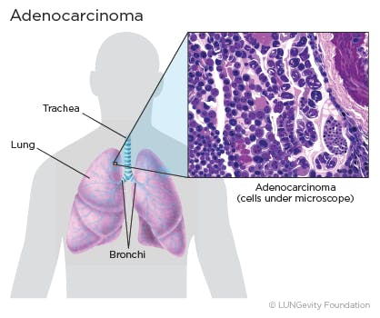
- Lung adenocarcinoma is a subtype of non-small cell lung cancer (NSCLC). Lung adenocarcinoma is categorized as such by how the cancer cells look under a microscope. Lung adenocarcinoma starts in glandular cells, which secrete substances such as mucus, and tends to develop in smaller airways, such as alveoli. Lung adenocarcinoma is usually located more along the outer edges of the lungs. Lung adenocarcinoma tends to grow more slowly than other lung cancers.
Lung adenocarcinoma accounts for 40% of all lung cancers. It is found more often in women. Younger people (aged 20-46) who have lung cancer are more likely to have lung adenocarcinoma than other lung cancers. Most lung cancers in people who have never smoked are adenocarcinomas.
Note that lung adenocarcinoma may not cause any symptoms, especially early on in its development and that the signs and symptoms are not specific to lung adenocarcinoma and may be caused by other conditions.
3 Lung squamous cell carcinoma ==> lung_scc :
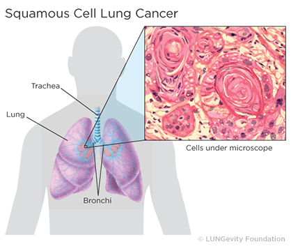
Squamous cell lung cancer, or squamous cell carcinoma of the lung, is one type of non-small cell lung cancer (NSCLC).Squamous cell lung cancer is categorized as such by how the cells look under a microscope. Squamous cell lung cancer begins in the squamous cells—thin, flat cells that look like fish scales when seen under a microscope. They line the inside of the airways in the lungs. Squamous cell lung cancer is also called epidermoid carcinoma
Squamous cell lung tumors usually occur in the central part of the lung or in one of the main airways (left or right bronchus). The tumor’s location is responsible for symptoms such as cough, trouble breathing, chest pain, and blood in the sputum. If the tumor grows to a large size, a chest X-ray or computed tomography (CT or CAT ) scan may detect a cavity in the lung. A cavity is a gas- or fluid-filled space within a tumor mass or nodule and is a classic sign of squamous cell lung cancer. Squamous cell lung cancer can spread to multiple sites, including the brain, spine and other bones, adrenal glands, and liver.
About 30% of all lung cancers are classified as squamous cell lung cancer. It is more strongly associated with smoking than any other type of non-small cell lung cancer. Other risk factors for squamous cell lung cancer include age, family history, and exposure to secondhand smoke, mineral and metal dust, asbestos, or radon.
Note that squamous cell lung cancer may not cause any symptoms, especially early on in its development and that the signs and symptoms are not specific to squamous cell lung cancer and may be caused by other conditions.
5. Preparing the tools
- pandas for data analysis.
- NumPy for numerical operations.
- Matplotlib/seaborn for plotting or data visualization.
- Scikit-Learn for machine learning modelling and evaluation.
- TensorFlow for bundles together Machine Learning and Deep Learning models and algorithms./Deep Learning Framework
import numpy as np # np is short for numpy
import pandas as pd # pandas is so commonly used, it's shortened to pd
import matplotlib.pyplot as plt
import seaborn as sns # seaborn gets shortened to sns
import tensorflow as tf
import os

# We want our plots to appear in the notebook
%matplotlib inline

## Models
from tensorflow.keras.models import Sequential

## Layers
from tensorflow.keras.layers import Conv2D
from tensorflow.keras.layers import MaxPool2D
from tensorflow.keras.layers import Flatten
from tensorflow.keras.layers import Dense
from tensorflow.keras.layers import Dropout #for Overfiting Problem

## Preprocessing
from tensorflow.keras.preprocessing.image import ImageDataGenerator
from tensorflow.keras.preprocessing.image import img_to_array
from tensorflow.keras.preprocessing.image import load_img
from tensorflow.keras.callbacks import EarlyStopping #for Overfiting Problem
from tensorflow.keras.utils import plot_model
from matplotlib.image import imread
import matplotlib.image as mpimg
from tensorflow.keras.preprocessing import image


## Model evaluators
from sklearn.metrics import confusion_matrix, classification_report
from sklearn.metrics import precision_score, recall_score, f1_score

#Load Model
from tensorflow.keras.models import load_model
6. Load Data
- This dataset contains 15,000 histopathological images with 3 classes. All images are 768 x 768 pixels in size and are in jpeg file format.
- The images were generated from an original sample of HIPAA compliant and validated sources, consisting of 750 total images of lung tissue (250 benign lung tissue, 250 lung adenocarcinomas, and 250 lung squamous cell carcinomas) and augmented to 15,000 using the Augmentor package.
- There are three classes in the dataset, each with 5,000 images, being :
- Lung benign tissue ==> lung_n
- Lung adenocarcinoma ==> lung_aca
- Lung squamous cell carcinoma ==> lung_scc
#load data direction
data_dir = 'E:\\Final Project\\lung_data_split'

#what our data include
os.listdir(data_dir)

train_data_dir = data_dir+'\\train\\'
val_data_dir = data_dir+'\\val\\'
test_data_dir = data_dir+'\\test\\'

os.listdir(train_data_dir)
7.Preparing the Data
7.1 Data Augmentation
- We will increase the size of the image training dataset artificially by performing some Image Augmentation techniques.
# Create Image Data Generator for Train Set
image_gen = ImageDataGenerator(
                               rescale=1./255,
                               shear_range=0.2,
                               zoom_range=0.2,
                               horizontal_flip=True
                              )

# Create Image Data Generator for Test/Validation Set
test_data_gen = ImageDataGenerator(rescale=1./255)
7.2 Loading the Images
train =image_gen.flow_from_directory(
                                     train_data_dir,
                                     target_size=(150,150),
                                     color_mode='rgb',
                                     class_mode='categorical',
                                     batch_size=32
                                    )

test =test_data_gen.flow_from_directory(
                                         test_data_dir,
                                         target_size=(150,150),
                                         color_mode='rgb',
                                         class_mode='categorical',
                                         batch_size=32,
                                         shuffle=False
                                        )
# setting shuffle as False just so we can later compare it with predicted values without having an indexing problem

valid =test_data_gen.flow_from_directory(
                                         val_data_dir,
                                         target_size=(150,150),
                                         color_mode='rgb',
                                         class_mode='categorical',
                                         batch_size=32,
                                        )
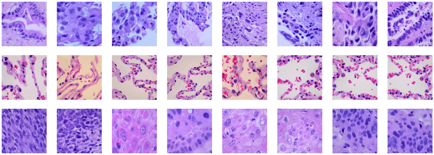
Look at some of the train set images
lung_aca_names = os.listdir(train_data_dir+'\\lung_aca\\')
lung_aca_names[:10]
lung_n_names = os.listdir(train_data_dir+'\\lung_n\\')
lung_n_names[:10]
lung_scc_names = os.listdir(train_data_dir+'\\lung_scc\\')
lung_scc_names[:10]
# parameters for the graph. The images will be in a 4x4 configuration
nrows = 8
ncols = 8

pic_index = 0 #index for iterating over images

#set up matplotlib figure
fig = plt.gcf()
fig.set_size_inches(ncols*4, nrows*4)

pic_index+=8

lung_aca_pic = [os.path.join(train_data_dir+'\\lung_aca\\', fname) for fname in lung_aca_names[pic_index-8:pic_index]]
lung_n_pic = [os.path.join(train_data_dir+'\\lung_n\\', fname) for fname in lung_n_names[pic_index-8:pic_index]]
lung_scc_pic = [os.path.join(train_data_dir+'\\lung_scc\\', fname) for fname in lung_scc_names[pic_index-8:pic_index]]


for i, img_path in enumerate(lung_aca_pic + lung_n_pic +lung_scc_pic):
    # setting up subplot. subplots start at index 1
    sub = plt.subplot(nrows, ncols, i + 1)
    sub.axis("off") #turning off axis. Don't show axis

    img = mpimg.imread(img_path)
    plt.imshow(img)
plt.show()

#1-Lung adenocarcinoma
#2-Lung benign tissue
#3-Lung squamous cell carcinoma
8.Convolutional Neural Network
- IT is an Artificial Neural Network that has the ability to pinpoint or detect patterns in the images. CNN architecture Example

- Image to see how CCN work
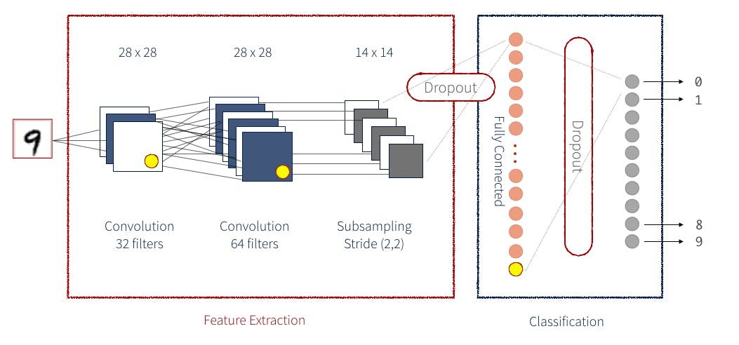
#Define the model Layers (Define The model)
model =Sequential()

# first convolution
model.add(Conv2D(32,(3,3),activation='relu',input_shape=(150,150,3)))
model.add(MaxPool2D(pool_size=(2,2)))

# second convolution
model.add(Conv2D(64,(3,3),activation='relu'))
model.add(MaxPool2D(pool_size=(2,2)))

# Third convolution
model.add(Conv2D(64,(3,3),activation='relu'))
model.add(MaxPool2D(pool_size=(2,2)))

# flatten before feeding into Dense neural network.
model.add(Flatten())

# 512 neurons in the hidden layer
model.add(Dense(512,activation='relu'))

model.add(Dropout(rate=0.4))

#3 = 3 different categories
    # softmas takes a set of values and effectively picks the biggest one. for example if the output layer has
    # [0.1,0.1,0.5], it will take it and turn it into [0,0,1]
model.add(Dense(3,activation='softmax'))

#Compiling the model

optmz = tf.keras.optimizers.Adam(learning_rate=3e-4, beta_1=0.9, beta_2=0.999, epsilon=1e-07, amsgrad=False,name='Adam')

model.compile(optimizer =optmz,loss="categorical_crossentropy",metrics=['accuracy'])
Getting a summary of the model built above.
model.summary()
Model: "sequential"
_________________________________________________________________
Layer (type)                 Output Shape              Param #
=================================================================
conv2d (Conv2D)              (None, 148, 148, 32)      896
_________________________________________________________________
max_pooling2d (MaxPooling2D) (None, 74, 74, 32)        0
_________________________________________________________________
conv2d_1 (Conv2D)            (None, 72, 72, 64)        18496
_________________________________________________________________
max_pooling2d_1 (MaxPooling2 (None, 36, 36, 64)        0
_________________________________________________________________
conv2d_2 (Conv2D)            (None, 34, 34, 64)        36928
_________________________________________________________________
max_pooling2d_2 (MaxPooling2 (None, 17, 17, 64)        0
_________________________________________________________________
flatten (Flatten)            (None, 18496)             0
_________________________________________________________________
dense (Dense)                (None, 512)               9470464
_________________________________________________________________
dropout (Dropout)            (None, 512)               0
_________________________________________________________________
dense_1 (Dense)              (None, 3)                 1539
=================================================================
Total params: 9,528,323
Trainable params: 9,528,323
Non-trainable params: 0
_________________________________________________________________
8.1 Fit the model
#Defining Callback list
early = EarlyStopping(monitor='val_loss',patience=2,mode='min')

#Fit The model
model.fit_generator(train,epochs=25,validation_data=valid)
Epoch 2/25
329/329 [==============================] - 289s 878ms/step - loss: 0.2608 - accuracy: 0.8943 - val_loss: 0.2166 - val_accuracy: 0.9113
Epoch 3/25
329/329 [==============================] - 270s 821ms/step - loss: 0.2037 - accuracy: 0.9188 - val_loss: 0.1838 - val_accuracy: 0.9210
Epoch 4/25
329/329 [==============================] - 277s 841ms/step - loss: 0.1859 - accuracy: 0.9284 - val_loss: 0.1579 - val_accuracy: 0.9370
Epoch 5/25
329/329 [==============================] - 284s 863ms/step - loss: 0.1673 - accuracy: 0.9350 - val_loss: 0.1489 - val_accuracy: 0.9413
Epoch 6/25
329/329 [==============================] - 308s 935ms/step - loss: 0.1607 - accuracy: 0.9356 - val_loss: 0.1804 - val_accuracy: 0.9240
Epoch 7/25
329/329 [==============================] - 308s 936ms/step - loss: 0.1313 - accuracy: 0.9491 - val_loss: 0.1405 - val_accuracy: 0.9377
Epoch 8/25
329/329 [==============================] - 307s 932ms/step - loss: 0.1245 - accuracy: 0.9526 - val_loss: 0.1126 - val_accuracy: 0.9527
Epoch 9/25
329/329 [==============================] - 303s 920ms/step - loss: 0.1251 - accuracy: 0.9510 - val_loss: 0.1431 - val_accuracy: 0.9450
Epoch 10/25
329/329 [==============================] - 303s 921ms/step - loss: 0.1064 - accuracy: 0.9587 - val_loss: 0.0765 - val_accuracy: 0.9717
Epoch 11/25
329/329 [==============================] - 300s 911ms/step - loss: 0.0875 - accuracy: 0.9657 - val_loss: 0.0680 - val_accuracy: 0.9760
Epoch 12/25
329/329 [==============================] - 384s 1s/step - loss: 0.0925 - accuracy: 0.9648 - val_loss: 0.0904 - val_accuracy: 0.9637
Epoch 13/25
329/329 [==============================] - 366s 1s/step - loss: 0.0723 - accuracy: 0.9730 - val_loss: 0.0613 - val_accuracy: 0.9760
Epoch 14/25
329/329 [==============================] - 249s 756ms/step - loss: 0.0788 - accuracy: 0.9678 - val_loss: 0.0723 - val_accuracy: 0.9740
Epoch 15/25
329/329 [==============================] - 201s 611ms/step - loss: 0.0582 - accuracy: 0.9794 - val_loss: 0.0633 - val_accuracy: 0.9753
Epoch 16/25
329/329 [==============================] - 201s 611ms/step - loss: 0.0617 - accuracy: 0.9758 - val_loss: 0.0596 - val_accuracy: 0.9790
Epoch 17/25
329/329 [==============================] - 204s 619ms/step - loss: 0.0482 - accuracy: 0.9835 - val_loss: 0.0713 - val_accuracy: 0.9753
Epoch 18/25
329/329 [==============================] - 202s 613ms/step - loss: 0.0477 - accuracy: 0.9825 - val_loss: 0.0637 - val_accuracy: 0.9737
Epoch 19/25
329/329 [==============================] - 202s 615ms/step - loss: 0.0387 - accuracy: 0.9853 - val_loss: 0.0260 - val_accuracy: 0.9920
Epoch 20/25
329/329 [==============================] - 203s 618ms/step - loss: 0.0358 - accuracy: 0.9866 - val_loss: 0.0504 - val_accuracy: 0.9833
Epoch 21/25
329/329 [==============================] - 203s 616ms/step - loss: 0.0410 - accuracy: 0.9856 - val_loss: 0.0635 - val_accuracy: 0.9720
Epoch 22/25
329/329 [==============================] - 202s 613ms/step - loss: 0.0391 - accuracy: 0.9858 - val_loss: 0.0294 - val_accuracy: 0.9890
Epoch 23/25
329/329 [==============================] - 202s 615ms/step - loss: 0.0321 - accuracy: 0.9895 - val_loss: 0.0441 - val_accuracy: 0.9807
Epoch 24/25
329/329 [==============================] - 202s 613ms/step - loss: 0.0318 - accuracy: 0.9884 - val_loss: 0.0293 - val_accuracy: 0.9873
Epoch 25/25
329/329 [==============================] - 202s 613ms/step - loss: 0.0376 - accuracy: 0.9875 - val_loss: 0.0265 - val_accuracy: 0.9910
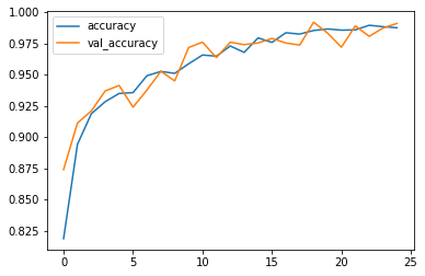
After 25th epochs , loss: 3.76% - accuracy: 98.75% - val_loss =2.65% and val_accuracy = 99.1%.
9.Evaluate
Display Data Frame , to show result
losses = pd.DataFrame(model.history.history)
losses
    loss    accuracy    val_loss    val_accuracy
0    0.406556    0.818762    0.282786    0.874000
1    0.260829    0.894286    0.216612    0.911333
2    0.203748    0.918762    0.183814    0.921000
3    0.185943    0.928381    0.157870    0.937000
4    0.167282    0.934952    0.148858    0.941333
5    0.160665    0.935619    0.180409    0.924000
6    0.131286    0.949143    0.140499    0.937667
7    0.124453    0.952571    0.112573    0.952667
8    0.125083    0.951048    0.143113    0.945000
9    0.106354    0.958667    0.076468    0.971667
10    0.087470    0.965714    0.067990    0.976000
11    0.092488    0.964762    0.090435    0.963667
12    0.072257    0.972952    0.061263    0.976000
13    0.078837    0.967809    0.072340    0.974000
14    0.058178    0.979429    0.063255    0.975333
15    0.061739    0.975810    0.059614    0.979000
16    0.048189    0.983524    0.071324    0.975333
17    0.047651    0.982476    0.063689    0.973667
18    0.038731    0.985333    0.026008    0.992000
19    0.035842    0.986571    0.050398    0.983333
20    0.041019    0.985619    0.063487    0.972000
21    0.039074    0.985810    0.029373    0.989000
22    0.032058    0.989524    0.044130    0.980667
23    0.031831    0.988381    0.029324    0.987333
24    0.037558    0.987524    0.026539    0.991000
Display some graphs to see if the model work good in training or not
losses[['loss','val_loss']].plot()
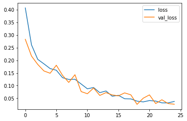
losses[['accuracy','val_accuracy']].plot()
9.1 Evaluating our model with Data that he didn't see before
Classification Report
We can make a classification report using classification_report() and passing it the true labels, as well as our models, predicted labels.
A classification report will also give us information of the precision and recall of our model for each class.
#Print classification Report

test_steps_per_epoch = np.math.ceil(test.samples / test.batch_size)

predictions = model.predict_generator(test, steps=test_steps_per_epoch)

predicted_classes = np.argmax(predictions, axis=1)

true_classes = test.classes

class_labels = list(test.class_indices.keys())

report = classification_report(true_classes, predicted_classes, target_names=class_labels)

print(report)
             precision    recall  f1-score   support

    lung_aca       0.98      0.99      0.99       500
      lung_n       1.00      1.00      1.00       500
    lung_scc       0.99      0.98      0.98       500

    accuracy                           0.99      1500
   macro avg       0.99      0.99      0.99      1500
weighted avg       0.99      0.99      0.99      1500
- Precision - Indicates the proportion of positive identifications (model predicted class 1) which were actually correct. A model which produces no false positives has a precision of 1.0.
- Recall - Indicates the proportion of actual positives which were correctly classified. A model which produces no false negatives has a recall of 1.0.
- F1 score - A combination of precision and recall. A perfect model achieves an F1 score of 1.0.
- Support - The number of samples each metric was calculated on.
- Accuracy - The accuracy of the model in decimal form. Perfect accuracy is equal to 1.0.
- Macro avg - Short for macro average, the average precision, recall and F1 score between classes. Macro avg doesn’t class imbalance into effort, so if you do have class imbalances, pay attention to this metric.
- Weighted avg - Short for weighted average, the weighted average precision, recall and F1 score between classes. Weighted means each metric is calculated with respect to how many samples there are in each class. This metric will favour the majority class (e.g. will give a high value when one class out performs another due to having more samples).
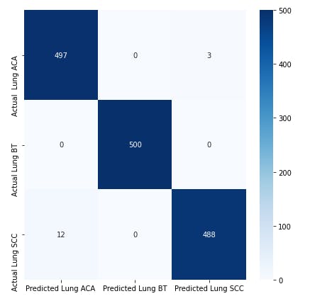
Confusion Matrix
A confusion matrix is a visual way to show where your model made the right predictions and where it made the wrong predictions (or in other words, got confused).
#Print confusion matrix

plt.subplots(figsize=(7,7))

cm = confusion_matrix(true_classes,predicted_classes)

cm_df =pd.DataFrame(cm,
                    columns=['Predicted Lung ACA ','Predicted Lung BT','Predicted Lung SCC'],
                    index=['Actual  Lung ACA ','Actual Lung BT','Actual Lung SCC'])

sns.heatmap(cm_df,annot=True,cmap="Blues", fmt='.0f');
#Save The Model
model.save("lung_cancer.h5")
9.2 Predict Some Images :
- Index 0 =Lung adenocarcinoma ==> lung_aca
- Index 1 =Lung benign tissue ==> lung_n
- Index 2 =Lung squamous cell carcinoma ==> lung_scc
# Index 1 = Lung benign tissue ==> lung_n
single_Lung_hist_n = "E:\\Final Project\\lung_data_split\\test\\lung_n\\lungn242.jpeg"

img = image.load_img(single_Lung_hist_n, target_size = (150, 150))
array = image.img_to_array(img)
x = np.expand_dims(array, axis=0)
test_image = model.predict_proba(x)
result = test_image.argmax(axis=-1)

if result ==[2]:
    print('Lung squamous cell carcinoma ')
elif result ==[0]:
    print('Lung Adenocarcinoma')
elif result ==[1]:
    print('Lung benign tissue ')
Lung benign tissue
10. Load Model
#Load Model
model_dir= 'lung_cancer.h5'

# loading using .h5 file
new_lung_model = tf.keras.models.load_model(
    "lung_cancer.h5",
    custom_objects=None,
    compile=True)
Great Job! We’ve just created a CNN model that can classify histopathological images as a Lung benign tissue or a Lung adenocarcinoma or a Lung squamous cell carcinoma with 99.1% accuracy after the 25th epochs.